Talking to each other, or just reacting to the same thing?

This post is about the paper Mutual information disentangles genuine interactions from shared environmental fluctuations, published in Physical Review Letters in 2021. You can also find a great viewpoint in APS’ Physics magazine written by Katie Newhall.

Around five years ago, I submitted the first of what would become a long series of papers at the intersection between information theory, stochastic processes, and statistical physics. It all started with a simple idea and what we thought would be a simple calculation (turns out, it wasn’t): what can we learn about the interactions between two systems if all we can observe is how they move together?

So, what better time than now to finally start writing about my own research? This will be the first in a series of (hopefully) divulgative pieces about the work I’ve done over the years, the ideas that started it, and what we have learned so far. If you want technicalities, just look for the section at the end!

To interact, or to not interact

Suppose you notice that two people’s moods seem to rise and fall together. When one is stressed, so is the other, and when one relaxes, so does the other. As you guess what may be going on, you might be tempted to conclude that these two people may be genuinely affecting each other - maybe they talk to each other, maybe one’s stress spills over into the other’s, maybe they wind each other up. But then, you might also consider the possibility that the may not be interacting at all. Rather, they could both be reacting, independently, to the same outside thing: the same stressful news cycle, the same looming deadline at the same shared job, the same bad weather. From the outside, watching only their moods, these two situations can look completely identical. And yet they are entirely different: in one case, breaking the connection between them would change everything. In the other, it would change nothing at all.

Here’s a more physical version of the same puzzle, which is surprisingly close to the mathematical model we ended up studying. Picture two dust particles floating in a still room, jittering around (you can think that the jittering comes from random collisions with air molecules, but it’s not important). Now suppose the room has a hidden thermostat that randomly flips between “warm” and “cool” — warmer means more jittering, cooler means less. The two particles never touch and don’t interact directly in any way. But because they share the same hidden thermostat, their motion still ends up looking very similar: watch one jitter more, and you can bet the other is jittering more too. If you didn’t know the thermostat existed, you might reasonably conclude these two particles were somehow talking to each other, rather than just following the same invisible temperature switches. You’d be wrong.

Temporal scales matter

The story above is a metaphor for a very real problem in science, which is also the research question behind the paper: if all you can observe is how two things move together, how do you tell whether they’re genuinely connected, or just both being pushed around by the same hidden, unobserved influence? Whenever researchers measure correlated activity between two neurons, two genes, or two ecological species, they face exactly this ambiguity: are these things actually coupled, or are they both just responding to something nobody measured? Getting it wrong means inferring a whole network of interactions that isn’t there, like a map of friendships between people who have never met.

To address this question from a quantitative perspective, we needed to strip it down to its bare essentials. We built a deliberately simple mathematical model of exactly this situation: two systems sharing a hidden environment that randomly switches back and forth between two states, invisible to us. We then studied a measure called mutual information, which captures how much information the two systems share with each other, regardless of the source (interactions, or shared environmental factors). Then we asked the question that turned out to be the key: does it matter how fast that hidden environment changes?

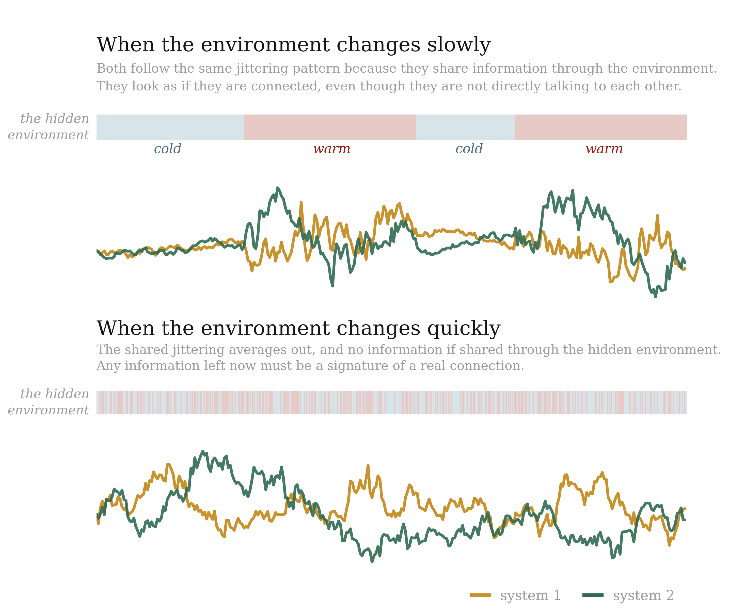
What we found. As it turns out, the difference between the temporal scales between the system and the environment matters enormously. Think about two cases: when the environment switches slowly, the thermostat stays “warm” for a long time, then “cool” for a long time. Or, similarly, the two people live in a world where the stressful news cycle is long and drawn out, or the looming deadline is far away. In this case, something remarkable happens: the two systems that spend long stretches of time under the same conditions end up looking like they are talking to each other. The correlations that the slow environmental changes produce can be just as strong as what a genuine interaction would give rise to. Our two friends look inseparable, and yet they may never have spoken.

The other case is the opposite: the news cycle keeps changing, the thermostat keeps flipping, the deadline keeps moving. In this scenario, we have shown that the shared influence averages out and the spurious correlation collapses. The two systems to “catch up” with each other. The two friends are still reacting to the same news, but the news is changing so quickly that they can’t stay in sync.

Why it’s useful. This gives you a test: whatever correlation survives fast switching cannot be blamed on the environment. Rather, it has to come from a real connection, if one exists at all. But there’s more: the two effects add up cleanly rather than tangling together when interactions are linear, meaning the two systems influence each other in a simple, proportional way. When they don’t, the two effects start interfering, and the neat separation breaks down. That turned out to be a rich problem in its own right, and a lot of my later work went into it — but that’s a story for another time.

Some technical details

We consider two stochastic processes $x_1(t)$ and $x_2(t)$ that share a common, randomly switching diffusion coefficient $D_{i(t)}$, where $i(t)$ jumps between two states ${-,+}$ with $D_+ > D_-$. Concretely, the dynamics can be written as the coupled Langevin equations

where $\xi_1, \xi_2$ are independent white noises. Here, $\tau$ is the relaxation timescale of the two systems, which sets how quickly they evolve, and $A_{12}, A_{21}$ are the linear interaction strengths between them. The switching process $i(t)$ is a two-state Markov process with transition rates $w_+$ and $w_-$, which set the average time spent in each state and so the environmental timescale $\tau_\text{env} = 1/(w_+ + w_-)$. The ratio $\tau_\text{env}/\tau$ is the key parameter that controls how much the environment contributes to the mutual information between $x_1$ and $x_2$.

To quantify how dependent $x_1$ and $x_2$ actually are, we first need to compute their joint probability distribution $p_{12}(x_1,x_2)$, which is the solution of the Fokker-Planck equation associated with the Langevin equations above. Even for this simple system, the Fokker-Planck equation is not analytically solvable outside of the fast- and slow-switching limits. In these limits, we then have to compute the mutual information,

where $p_1(x_1)$ and $p_2(x_2)$ are the marginal distributions. The reason why $I$ is useful is that it captures all statistical dependencies between $x_1$ and $x_2$, and it is zero exactly when $x_1$ and $x_2$ are statistically independent. A positive value of $I$ indicates that knowing one variable provides information about the other regardless of whether that dependency is linear, and regardless of its origin. $I$, in general, is hard to compute, and we resolve to bounds to study it. Luckily, the bounds saturate in some regimes, allowing us to make exact statements about the mutual information in those limits.

The key result concerns two cases, depending on the relative timescales of the environment and the system. Let’s start in the absence of any real interaction ($A_{12} = A_{21} = 0$) and study $I_\text{env}$, the mutual information coming purely from the shared environment.

• Fast switching ($\tau_\text{env} \ll \tau$): $x_1$ and $x_2$ each effectively experience the environmental average of the diffusion coefficient. Thus, if there are no real interactions, they become statistically independent, and $I \to 0$.
• Slow switching ($\tau_\text{env} \gg \tau$): $x_1$ and $x_2$ spend long stretches of time under the same fixed $D_i$, producing genuine statistical dependence. In suitable limits (when the environmental states are “infinitely different” from each other) the mutual information coming from the environment can be computed exaclty and approaches its maximum possible value: the entropy of the switching process itself, i.e. how uncertain you are, at any given moment, about which environmental state you’re in.

When real, linear interactions between $x_1$ and $x_2$ are added on top of this ($A_{12}, A_{21} \neq 0$), the two contributions to $I$ don’t get mixed together arbitrarily, Rather, they add: $I_\text{tot} = I_\text{int} + I_\text{env}$. In the fast-switching limit, where the environmental piece vanishes entirely, whatever mutual information remains is coming from the real interaction alone, and only from it. That’s the disentangling in the title of the paper: pushing the environment into the fast-switching regime isolates the genuine coupling from the spurious, environment-induced one.

Read the paper (Phys. Rev. Lett. 127, 228301) · arXiv preprint