

Fast things, slow things, and information
This post is about two papers: Information propagation in multilayer systems with higher-order interactions across timescales, published in Physical Review X in 2024, and Information propagation in Gaussian processes on multilayer networks, published in the Journal of Physics: Complexity in 2024. A comprehensive review titled Stochastic processes with multiple temporal scales: timescale separation and information was then published in Journal of Statistical Mechanics: Theory and Experiment in 2025.
Over the years, I kept running into the same structure in problems that, at first sight, had little to do with each other. Two particles reacting to a hidden environment that changes slowly over time. A system that gets used to a repeated signal because a slow internal memory builds up underneath its fast response. A patch of cortex that is constantly driven by slow inputs coming from the rest of the brain. Every time, something changing quickly was sitting on top of something whose dynamics was slower, and every time the difference in speed shaped how much information the different parts ended up sharing. At some point, we decided to stop solving these problems one at a time and to ask a more general question: how does information travel through a system whose parts live on very different timescales?
Who is pushing whom
Let’s start from an everyday example: a city, its roads, and its traffic. Traffic changes within minutes, as cars come and go and jams form and dissolve. Roads change much more slowly. For example, a road closed for works can stay closed for months. These are two processes living on very different timescales, and they influence each other in both directions.
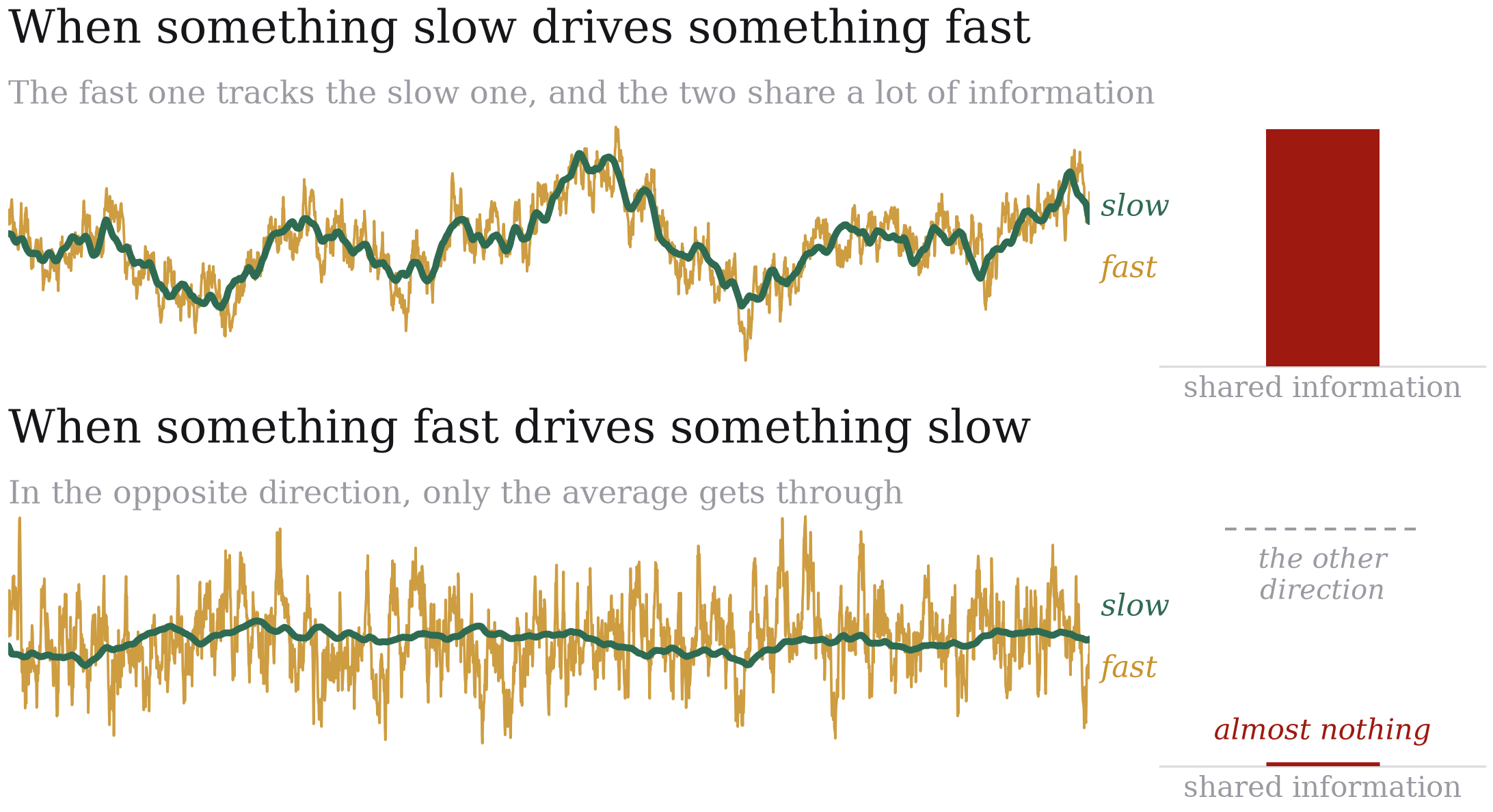
First, the roads shape the traffic. Close a road, and within minutes or hours the cars find other routes and the jams move with them. So, if you opened a map of the traffic right now, you could probably guess where the road works are. What this means is that, by watching the fast process, you can tell something about the current state of the slow one. Or, as we would say, you have information about it.
But the traffic also shapes the roads. Every car wears the asphalt a little, and the busiest roads are the ones that end up needing repairs. This influence is just as real as the other one. And yet, if I showed you how worn a road is, could you tell me how many cars are driving on it right now? You probably can’t. The wear is the result of years of traffic, and what it reflects is the average over all of them, not what is happening minute by minute.
To make this precise, we need a way to measure how much observing one thing tells you about another. This is what mutual information does: it is zero when knowing one thing tells you nothing about the other, and it grows the more one can be predicted from the other. But here’s the catch: the mutual information is also symmetric, meaning that whatever the traffic tells you about the roads, the roads tell you about the traffic. And yet, even if the two influences are equally real, only one of them lets you read the present state of the other. How can this be?
What our example shows is where this shared information comes from. And it’s all about timescales: knowing which roads are closed tells you where the cars are now, and the other way around, because the traffic changes much faster than the roads. The traffic wearing out the asphalt adds nothing to this information, no matter how much it changes the roads. When the slow pushes the fast, information appears. But when the fast pushes the slow, there is an influence without any information.
Layers, clocks, and the propagation of information
In these two papers (plus the review), we made this idea general. We describe a system as a stack of layers, each one with its own clock. Think of layers as a hierarchy of timescales: molecules that change within milliseconds, the cells they live in, whole populations of cells, and an environment that changes over days. Inside each layer, the units interact with each other as in a network. Across layers, the influence can be more complicated, and what typically happens is that the state of one layer can change the rules of the game in another, making for instance some transitions easier and others harder. Physicists call these higher-order interactions, because they act on the connection between two units rather than on a single unit. A road closure does exactly this, because it doesn’t move any car but rather it changes which routes are available to all of them.
The breakthrough came when we realized that, if the clocks of the different layers tick on sufficiently different timescales, this problem could be solved in general. The result boils down to three rules:
- When a slow layer regulates a faster one, it creates information: the fast layer settles around the current state of the slow one and becomes a record of it.
- When a fast layer pushes a slower one, it creates no information on its own, because only its average gets through.
- Once created, information can be propagated. If the fast layer that holds information about a slow one pushes a third layer in turn, it can pass that information along, as long as the third layer is still faster than the source.
In our traffic example, the third rule looks like the following. Think about the air quality in a quiet side street, which changes over a few days. If road works on the main road divert the traffic through that street, the air there gets worse. So the air quality of the side street ends up carrying information about the road works, even though the road works never touched the air directly. The traffic passed the information on.
Putting the three rules together, you can draw a map of which parts of a system share information with which, just by looking at who is connected to whom and at how fast each part is, without solving any equation. Importantly, this map is not the map of who influences whom. Two parts can push each other around and share no information at all, while two parts that never interact directly can end up sharing a lot. And what made this result particularly interesting is that it is not limited to a specific model: it holds for any system that can be described as a stack of layers with different clocks, whether the layers are discrete or continuous, and whether the interactions are pairwise or higher-order.
Same behavior, different information
Let’s go back to habituation, where, as they adapt to a signal that keeps arriving, many biological systems respond strongly at first and then less and less. A minimal circuit that does this has three parts: a receptor that receives the signal, a fast response that follows the receptor, and a slow storage that builds up and acts as a memory. The storage can then quiet the circuit in two ways, either by acting on the response directly, or by acting on the receptor upstream.
If you look at how the two circuits behave, they are very similar. In both, the response gets weaker at every repetition of the signal while the storage grows, and the only visible difference is whether the activity of the receptor drops as well. Our framework, however, shows that their information is very different. In fact, when the storage acts on the response, the storage and the receptor share no information at all, showing that the memory does its job without knowing anything about what the receptor is doing. When the storage acts on the receptor, every part of the circuit shares information with every other one. So information can tell apart two mechanisms that look almost the same from the outside.
Shared environments
The general rules we derived essentially explained several of our previous results, including the one that got us started on information in the first place. Take two systems that never interact, but are both regulated by the same slow environment, like the grains of dust or the two friends from my first paper on information theory. By the first rule, the environment creates information in each of them, and as a consequence the two systems end up sharing information with each other, even though they never interacted. When the environment acts strongly, this shared information approaches the entropy of the environment, which measures how unpredictable its state is.
Why it’s useful. In real systems, we rarely know how all the parts are connected, and often this is exactly what we want to find out. The information shared between different parts, on the other hand, can in principle be estimated from recordings of their activity, as long as the recordings are precise enough in time. The three rules connect the two.
Since a fast part pushing a slower one creates no information on its own, whenever two parts with different clocks share information, we know that somewhere there has to be something slower regulating something faster. Thus, together with how fast each clock is, the pattern of shared information can be used to understand how the different parts of a system operating on multiple temporal scales are connected. More broadly, grouping the parts of a complex system by how fast they are, and treating each group as a layer, could be a way to look at the information structure of systems that are far too complicated to model in detail.
After years of solving problems one at a time, with this framework we were finally able to put all the pieces of the puzzle together. The three rules are simple, but they are general and they explain a lot of what we had seen before. When we started, we were thinking about a few specific systems, but ended up with a framework that explains how information is generated and propagated in any system whose parts live on well-separated temporal scales. And, even though I was focusing on molecules and neurons, around that same time it turned out that the same separation of timescales could be applied to a completely different problem: ecology, where the fast and the slow are the individuals exploring a landscape and the populations that settle in it. That’s the story for next time.
Some technical details
The general framework. Consider \(N\) layers, each a network of \(M_\mu\) nodes with its own internal dynamics — master equations, random walks — and its own timescale, ordered as \(\tau_1 < \tau_2 < \dots < \tau_N\). In the PRX paper, layers are coupled by triadic higher-order interactions: the state of node \(k\) in layer \(\mu\) modulates the transition rates along the edge \(i \to j\) of layer \(\nu\), encoded in tensors \(C^{\mu\nu}\) that split into direct contributions (fast to slow) and feedback contributions (slow to fast). In the limit of separated timescales, the joint probability factorizes as
\[p_{1,\dots,N}(t) = p^{\text{eff}}_N(t) \prod_{\mu=1}^{N-1} p^{\text{st,eff}}_{\mu \vert \rho(\mu)},\]where only the slowest layer retains a genuine time dependence, and every other layer sits in an effective stationary state conditioned on \(\rho(\mu)\) — the set of slower layers that reach \(\mu\) through a feedback link or through an admissible propagation path. Faster layers enter each conditional only through effective operators, averaged over their own stationary states. This factorization is where the three principles come from: feedback interactions from slow to fast generate mutual information, because the fast layer’s conditional state depends explicitly on the slow one; direct interactions from fast to slow generate none, because they enter the slow dynamics only through averages; and direct links can relay feedback-generated information to further layers along the paths that survive in \(\rho\). The pairwise mutual information between layers, arranged into a matrix \(I_{\mu\nu}\), is then fixed entirely by the topology of the couplings and the ordering of the clocks.
The Gaussian case. The second paper works out the continuous, exactly solvable version: multilayer Ornstein–Uhlenbeck processes
\[\tau_\mu \dot{x}^i_\mu = -\left(x^i_\mu - \theta^i_\mu\right) + \sum_j A^{ij}_{\mu\mu} \left(x^j_\mu - \theta^j_\mu\right) + \sum_{\nu \neq \mu} \sum_j A^{ij}_{\mu\nu} \left(x^j_\nu - \theta^j_\nu\right) + \sqrt{2 D^i_\mu}\, \xi^i_\mu,\]with ordinary pairwise edges between layers and a stationary covariance given by a Lyapunov equation. In the timescale-separation limit the joint Gaussian factorizes hierarchically, exactly as above: a slow layer feeding a fast one leaves the fast layer’s conditional mean a linear function of the slow state — this dependence is the mutual information — while the reversed coupling leaves the layers statistically independent no matter how strongly it shapes the dynamics. The same three principles hold, showing that no higher-order structure is needed for them. On top of this, the paper studies the interplay between information and stability: with random Gaussian couplings inside each layer, a layer destabilizes when the spread of its couplings reaches a critical value. Pushing the slow layer that generates information toward its edge of stability increases the mutual information between all layers, together with its variability across realizations of the couplings; pushing instead the faster layer that relays it gives a smaller increase on average, with larger fluctuations of the relayed entries.
We then generalized this to any Fokker-Planck operator in a self-contained overview of the timescale-separation methods behind these results, Stochastic processes with multiple temporal scales: timescale separation and information, published in Journal of Statistical Mechanics in 2025.
Phys. Rev. X 14, 021007 (2024) · J. Phys. Complex. 5, 045004 (2024) · arXiv preprint (PRX) · arXiv preprint (J. Phys. Complex.)